Understanding Neural Networks and KE Sieve
A detailed approach to show how KE Sieve is equivalent to a neural network
As we have shown in previous posts, we can use the KE Sieve algorithm in most places where we need a neural network.
We have theoretical proof that the KE Sieve algorithm creates hyper dimensional planes that are equivalent to planes created by neural networks. The only difference is that the neural network finds these planes through an iterative approach using back propagation where the KE Sieve approach does it no iteratively, thus avoiding the training time.
But we wanted to prove this visually using a toy dataset.
First let's discuss a simple feedforward neural network:
Input Layer
Assume you have 2 inputs: x1 and x2. This could represent a 2-dimensional input vector.
Hidden Layer
Let's say there's one hidden layer with 2 neurons.
Each neuron in this layer will have its weights and biases. Let's denote the weights for the first neuron as w11 and w12, and for the second neuron as w21 and w22. The biases for the first and second neuron will be b1 and b2 respectively.
The output from the first neuron before activation would be: z1=w11x1+w12x2+b1
Similarly, the output from the second neuron before activation would be: z2=w21x1+w22x2+b2
Activation Function
Neural networks typically use an activation function to introduce non-linearity. Common choices are the sigmoid, ReLU (Rectified Linear Unit), tanh, etc.
For simplicity, let's use the sigmoid function, denoted as
\(σ(z)=1/(1+e^{-z})\)So, the activated outputs from our two neurons will be:
a1=σ(z1)
a2=σ(z2)
Output Layer
Let's assume a single output neuron for this layer.
This neuron will take the activated outputs from the hidden layer as input. Let's use weights v1 and v2 and bias b0 for this neuron.
The output of this neuron before activation would be: z0=v1a1+v2a2+b0
Using the sigmoid activation again: output=σ(z0)
For every neuron, if we consider the equation before the activation function, it's a linear combination of the inputs (in case of 2 inputs it's a plane in 3D space). So for our two neurons in the hidden layer, the plane equations would be: w11x1+w12x2+b1=0
w21x1+w22x2+b2=0
Each of these planes divides the input space into two halves, and the decision boundary will depend on the combination of these planes and the activation functions used.
So as we can see, every neuron in a neural network can be represented as hyper dimensional plane. So what the neural network does is, learn the weights and biases of this plane over multiple iterations and using back propagation.
Can we represent these hyperdimensional planes on a 2D system so that we can visualize what is happening? Turns out we can, by only choosing 2 of the 784 dimensions and plot them on 2D.
system
Lets take the MNIST dataset and do the following experiment:
Train a small neural network.
At each epoch, take the weights and biases and draw the planes in a 2D system and visualize how the planes are separating the training points.
Repeat for each epoch and observe if the planes are doing a better job of separating the training points.
Experiment results:
Neural network architecture used:
Model: "sequential_1"
_________________________________________________________________
Layer (type) Output Shape Param #
=================================================================
flatten_1 (Flatten) (None, 784) 0
dense_3 (Dense) (None, 26) 20410
dense_4 (Dense) (None, 10) 270
=================================================================
Total params: 20,680
Trainable params: 20,680
Non-trainable params: 0
To visualize each training step we used following method-
In each step we compute distance vector and then apply PCA with only 2 components.
We solve this 2d vector using linear regression to obtain a line equation and plot that line. Randomly we scatter few points of each class to get an idea how each plane is getting adjusted over consecutive epoch.
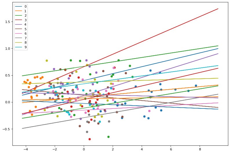
First plot is without training and random weights assigned.
Here we see the points and planes are random. Lets observe through a series of epochs how the planes move and separate the points. The output of 20 epochs is show below as a series of images.

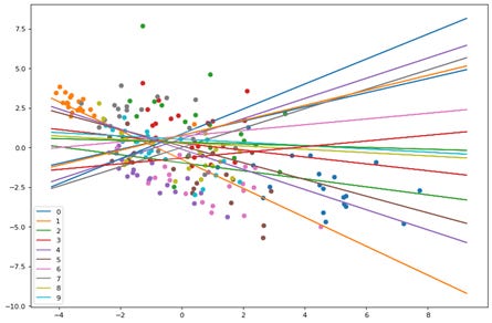
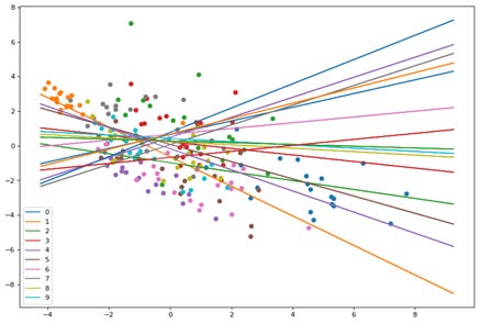
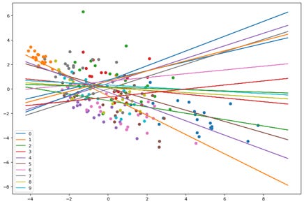
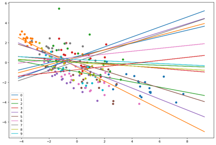
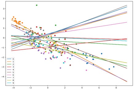
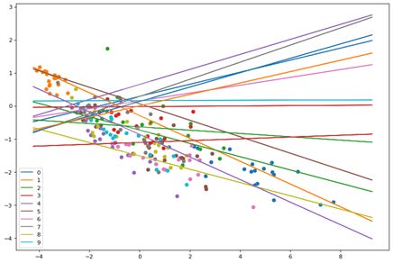
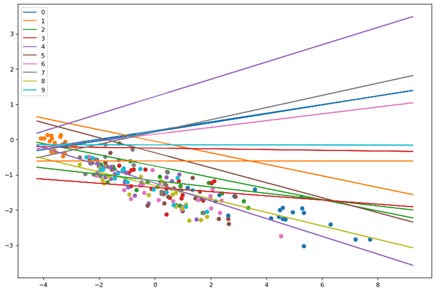
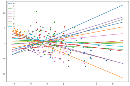
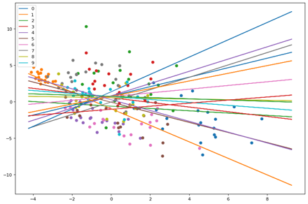
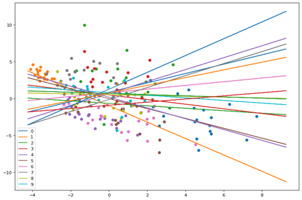

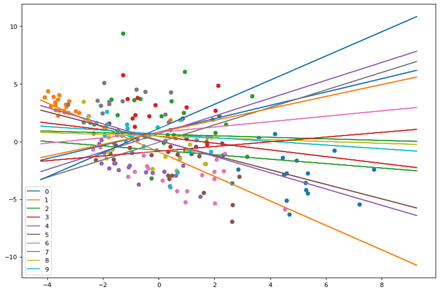
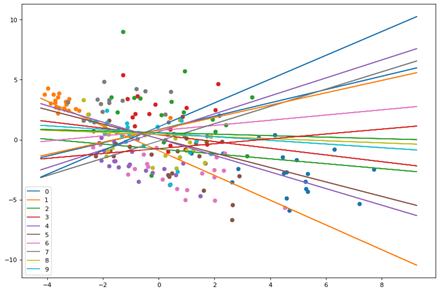
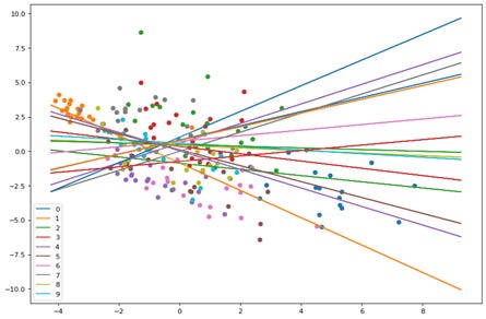
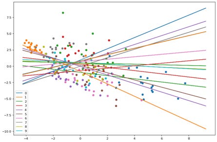
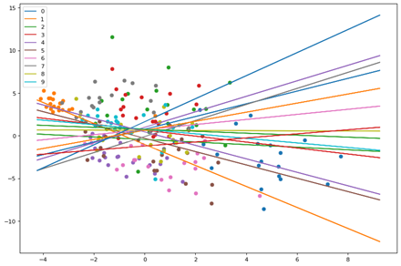
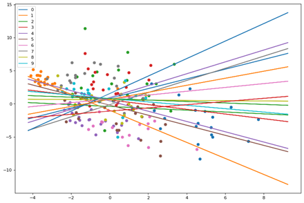
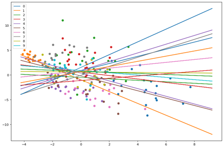
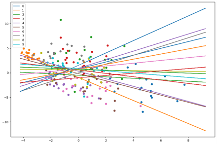
As you can clearly see, the planes are adjusting with each epoch to separate out the points and by the 20th epoch each neuron(plane) has some distinguishing character.
In the next article we will see how KE Sieve creates planes for the same problem.
Disclaimer:
The NN by using the Back propagation algorithm does its work differently from PCA. The NN tries to separate the classes by using hyperplanes. While the PCA is a statistical method which tries to determine the “Principle Components” in a multivariate (ie multi dimensional data). In this case the PCA chooses only two (“principle”) components (variables) say u and v which are linear combinations of the 784 dimensions that is MNIST data. So the plots are in u, v space. We have done the PCS just so that we can visualize the approximation of the space in 2D.


